Lecture 4: Monday, August 26, 2013

We have seen that the circle $S^1(\mathbb R)$ and the sphere $S^2(\mathbb R)$ can each be defined by a single equation, namely $u^2 + w^2 = r^2$ and $u^2 + v^2 + w^2 = r^2$ , respectively. However, the real projective line $\mathbb P^1(\mathbb R) \simeq S^1(\mathbb R)$ while the complex projective line $\mathbb P^1(\mathbb C) \simeq S^2(\mathbb R)$ , so can we think of the projective line $\mathbb P^1(K)$ as being defined by a single equation for any field $K$ ? And why do we call this a “line” anyway? In this lecture, we answer these questions and more.

Nonsingular Projective Varieties

Let’s begin with the precise language of projective varieties from algebraic geometry. We will be very technical in this first half of the lecture.

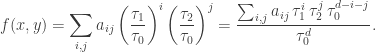
Let $K$ denote either $\mathbb Q$ , $\mathbb R$ , or $\mathbb C$ , even though the definitions hold for any number field. A subset in the form
$V(K) = \left \{ P \in \mathbb P^n(K) \ \biggl| \ F_k(P) = 0 \ \text{for} \ k = 1, \, 2, \, \dots, \, m \right \}$
is called a non-singular, irreducible, projective variety of dimension $d$ if the following axioms hold:

Homogeneity: Each $F_k$ is homogeneous polynomial of degree $e_k$ , that is, $F_k \bigl( \lambda \, \tau_1, \ \dots, \ \lambda \, \tau_n, \ \lambda \, \tau_0 \bigr) = \lambda^{e_k} \cdot F_k \bigl( \tau_1, \ \dots, \ \tau_n, \ \tau_0 \bigr)$ for all nonzero $\lambda \in K$ .

Nonsingularity: The $m \times (n+1)$ matrix
$\left[ \begin{matrix} \dfrac {\partial F_1}{\partial \tau_1}(P) & \cdots & \dfrac {\partial F_1}{\partial \tau_n}(P) & \dfrac {\partial F_1}{\partial \tau_0}(P) \\[15pt] \dfrac {\partial F_2}{\partial \tau_1}(P) & \cdots & \dfrac {\partial F_2}{\partial \tau_n}(P) & \dfrac {\partial F_2}{\partial \tau_0}(P) \\[15pt] \vdots & \ddots & \vdots & \vdots \\[15pt] \dfrac {\partial F_m}{\partial \tau_1}(P) & \cdots & \dfrac {\partial F_m}{\partial \tau_n}(P) & \dfrac {\partial F_m}{\partial \tau_0}(P) \end{matrix} \right]$
has rank $m$ for each $P \in \mathbb P^n(\mathbb C)$ satisfying $F_1(P) = F_2(P) = \cdots = F_m(P) = 0$ .

Irreducibility: With $S(e) \subseteq K[\tau_1, \dots, \tau_n, \tau_0]$ being the set of homogeneous polynomials $F(\tau_1, \dots, \tau_n,\tau_0)$ of degree $e$ , the set
$I(V) = \displaystyle \bigoplus_{e=0}^\infty \left \{ F(\tau_1, \dots, \tau_n,\tau_0) \in S(e) \, \biggl| \ F(P) = 0 \ \text{for all} \ P \in V(K) \right \}$
is a prime ideal in the graded polynomial ring $S = \displaystyle \bigoplus_{e = 0}^\infty S(e)$ . That is, since we have the product $S(e_1) \cdot S(e_2) \subseteq S(e_1 + e_2)$ , if $F \in S(e_1)$ and $G \in S(e_2)$ are homogeneous polynomials such that the product $F \cdot G \in I(V) \cap S(e_1 + e_2)$ , then either $F \in I(V) \cap S(e_1)$ or $G \in I(V) \cap S(e_2)$ .

Dimension: The integer $d = n - m$ is the number $n$ of homogeneous coordinates $\tau_k$ minus the number $m$ of hypersurfaces $F_k = 0$ .

Here, I’ve given ad hoc definitions to match the situations we’ll focus on in this class. If you wish to see the most general framework, I’d suggest reading through Hartshorne’s Algebraic Geometry.

If $d =$ 1, 2 or 3, we say that the non-singular, irreducible, projective variety $V: \, F_1 = F_2 = \cdots = F_m = 0$ is a curve, a surface, or a 3-fold, respectively. In this course, we will only be concerned with curves and surfaces.

Affine vs. Projective Curves

In order to gain some intuition with these definitions, we begin with the simplest case: when $V: F = 0$ is just defined by one equation. We continue to denote $K$ as either $\mathbb Q$ , $\mathbb R$ , or $\mathbb C$ .

Say that we have an irreducible polynomial $f(x,y)$ with $K$ -rational coefficients, that is, $f(x,y) = \sum_{i,j} a_{ij} \, x^i \, y^j$ where $a_{ij} \in K$ . The collection of affine points $(x,y) \in \mathbb A^2(K)$ such that $f(x,y) = 0$ is called an affine curve.

The degree of the polynomial is the largest $d = i+j$ such that $a_{ij} \neq 0$ . An example of such a polynomial is $f(x,y) = y^2 - \left( a_d \, x^d + a_{d-1} \, x^{d-1} + \cdots + a_1 \, x + a_0 \right)$ where $d \geq 2$ is an integer.

Make the substitution $x = \tau_1/\tau_0$ and $y = \tau_2/\tau_0$ so that we find the polynomial
$f(x,y) = \displaystyle \sum_{i,j} a_{ij} \left( \dfrac {\tau_1}{\tau_0} \right)^i \left( \dfrac {\tau_2}{\tau_0} \right)^j = \dfrac {\sum_{i,j} a_{ij} \, \tau_1^i \, \tau_2^j \, \tau_0^{d-i-j}}{\tau_0^d}.$
We define the homogenization of $f(x,y)$ to be the homogeneous polynomial of degree $d$ which occurs in the numerator above: $F(\tau_1,\tau_2,\tau_0) = \sum_{i,j} a_{ij} \, \tau_1^i \, \tau_2^j \, \tau_0^{d-i-j}$ . Note that by construction $f(x,y) = F(x,y,1)$ and $F(\tau_1,\tau_2,\tau_0) = \tau_0^d \cdot F(x,y,1)$ . The collection of points $(\tau_1:\tau_2:\tau_0) \in \mathbb P^2(K)$ such that $F(\tau_1,\tau_2,\tau_0) = 0$ is called a projective curve. As an example, if $f(x,y) = y^2 - \left( a_d \, x^d + a_{d-1} \, x^{d-1} + \cdots + a_1 \, x + a_0 \right)$ then its homogenization is
$F(\tau_1,\tau_2,\tau_0) = \tau_2^2 \, \tau_0^{d-2} - \left( a_d \, \tau_1^d + a_{d-1} \, \tau_1^{d-1} \, \tau_0 + \cdots + a_1 \, \tau_1 \, \tau_0^{d-1} + a_0 \, \tau_0^d \right).$

The notation $E: f(x,y) = 0$ in terms of the affine curve is shorthand for the collection of projective points:
$E(K) = \left \{ \, (\tau_1:\tau_2:\tau_0) \in \mathbb P^2(K) \, \biggl| \, F(\tau_1,\tau_2,\tau_0) = 0 \, \right \}.$
Recall that we have an injective map $\mathbb A^2(K) \to \mathbb P^2(K)$ which sends 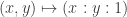$(x,y) \mapsto (x : y : 1)$ , so we may break the set above into two pieces:
$E(K) = \left \{ (x:y:1) \in \mathbb P^2(K) \, \biggl| \, f(x,y) = 0 \right \} \cup \left \{ (x:y:0) \in \mathbb P^2(K) \, \biggl| \, F(x,y,0) = 0 \right \}.$
The first set is essentially the collection of affine points, whereas the second set consists of those “points at infinity.”

Example

We work through an example as a precursor to elliptic curves.

Proposition.
Consider the curve $E: y^2 + a_1 \, x \, y + a_3 \, y = x^3 + a_2 \, x^2 + a_4 \, x + a_6$ where $a_i \in K$ . Then we have
$E(K) = \left \{ \, (x:y:1) \in \mathbb P^2(K) \, \biggl| \, y^2 + a_1 \, x \, y + a_3 \, y = x^3 + a_2 \, x^2 + a_4 \, x + a_6 \, \right \} \cup \{ (0:1:0) \}.$

We denote $\mathcal O = (0:1:0)$ as the “point at infinity” on $E$ .

Proof: Let $f(x,y) = y^2 + a_1 \, x \, y + a_3 \, y - x^3 - a_2 \, x^2 - a_4 \, x - a_6$ . (Note that this has degree $d = 3$ .) Make the substitution $x = \tau_1/\tau_0$ and $y = \tau_2/\tau_0$ so that we find the homogeneous polynomial
$F(\tau_1,\tau_2,\tau_0) = \tau_2^2 \, \tau_0 + a_1 \, \tau_1 \, \tau_2 \, \tau_0 + a_3 \, \tau_2 \, \tau_0^2 - \tau_1^3 - a_2 \, \tau_1^2 \, \tau_0 - a_4 \, \tau_1 \, \tau_0^2 - a_6 \, \tau_0^3.$
We have
$E(K) = \left \{ \, (x:y:1) \in \mathbb P^2(K) \, \biggl| \, f(x,y) = 0 \, \right \} \cup \left \{ (x:y:0) \in \mathbb P^2(K) \, \biggl| \, F(x,y,0) = 0 \right \}.$
Since $F(x,y,0) = -x^3$ we find that the collection of points at infinity consists of just the equivalence class $(x:y:0) = (0:y:0) = (0:1:0)$ . $\square$

Non-Singular Projective Curves

Say that we have a homogeneous polynomial $F(\tau_1, \tau_2, \tau_0)$ of degree $d$ with coefficients in $K$ . We define a projective curve $E$ to be the collection of all projective points $(\tau_1:\tau_2:\tau_0) \in \mathbb P^2(K)$ such that $F(\tau_1,\tau_2,\tau_0) = 0$ . We say $E$ is a non-singular projective curve if the gradient
$\nabla F(\tau_1,\tau_2,\tau_0) = \left( \dfrac {\partial F}{\partial \tau_1}, \ \dfrac {\partial F}{\partial \tau_2}, \ \dfrac {\partial F}{\partial \tau_0} \right)$
does not vanish for any projective point 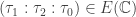$(\tau_1:\tau_2:\tau_0) \in E(\mathbb C)$ . This is an example of a non-singular, projective variety of dimension $d = 1$ . (Note that we have replaced $K$ by $\mathbb C$ .) Any projective point $P \in E(K)$ such that $\nabla F(P) = (0,0,0)$ is called a singular point. If $E$ is a nonsingular projective curve, its genus is the nonnegative integer $g(E) = (d-1) \, (d-2)/2$ .

Example: Non-Singular Projective Curve

We show a fundamental result about affine and projective lines.

Proposition.
Consider the curve $L: a \, x + b \, y + c = 0$ . Then $L$ is a nonsingular projective curve of genus $g(L) = 0$ .

Proof: We check that $L$ is a nonsingular projective curve by using homogeneous coordinates. Upon substituting $x = \tau_1 / \tau_0$ and $y = \tau_2 / \tau_0$ , we find the expression $f(x,y) = a \, x + b \, y + c = \dfrac {a \, \tau_1 + b \, \tau_2 + c \, \tau_0}{\tau_0}$ so denote the polynomial $F(\tau_1, \tau_2, \tau_0) = a \, \tau_1 + b \, \tau_2 + c \, \tau_0$ . Its gradient is $\nabla F(\tau_1, \tau_2, \tau_0) = \left( a, \, b, \, c \right) \neq (0,0,0)$ . Hence $L$ has no nonsingular points. Since $F(\tau_1, \tau_2, \tau_0)$ has degree $d = 1$ , we see that the genus of $L$ is $g(L) = (d-1) \, (d-2) / 2 = 0$ . $\square$

Note that a line $L$ is a subset of $\mathbb P^2(K)$ . In fact, we have an embedding 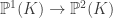$\mathbb P^1(K) \to \mathbb P^2(K)$ which sends $\left( \tau_1 : \tau_2 \right) \mapsto \left( \tau_1 : \tau_2 : 0 \right)$ ; so that we may identify $\mathbb P^1(K)$ as a line as well:
$\mathbb P^1(K) \simeq \left \{ (\tau_1 : \tau_2 : \tau_0) \in \mathbb P^2(K) \ \biggl | \ \tau_0 = 0\right \}.$
Since $\mathbb P^1$ is a line, it has genus $g(\mathbb P^1) = 0$ . We think of this line as the “line at infinity.”

In particular, if 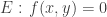$E: \, f(x,y) = 0$ is a curve, then the set $\left \{ (x:y:0) \in \mathbb P^2(K) \, \bigl| \, F(x,y,0) = 0 \right \}$ where $F(\tau_1, \tau_2, \tau_0) = \tau_0^d \cdot f \left( \tau_1/\tau_0, \ \tau_2/\tau_0 \right)$ is simply the intersection of the “line at infinity” with the projective curve $E$ . If $f(x,y)$ is a polynomial of degree $d$ , then this set consists of only $d$ projective points (counting multiplicity).

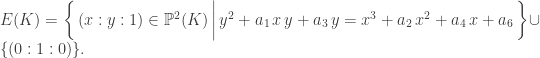
Example: Singular Projective Curve

For the final example, we discuss what happens when the curve is singular. Following Cassels’s classic text Lectures on Elliptic Curves, let’s consider the cubic curve $C: x^2 - y^2 = \left( x - 2 \, y \right) \left( x^2 + y^2 \right)$ .

Upon denoting $x = \tau_1 / \tau_0$ and $y = \tau_2 / \tau_0$ , we find the projective curve $F(\tau_1, \tau_2, \tau_0) = 0$ in terms of the homogeneous polynomial
$F(\tau_1, \tau_2, \tau_0) = \left( \tau_1^2 - \tau_2^2 \right) \tau_0 - \left( \tau_1 - 2 \, \tau_2 \right) \left( \tau_1^2 + \tau_2^2 \right).$
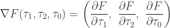
This is not a nonsingular projective curve. To see why, we compute the singular points. We have the partial derivatives
$\begin{aligned} \dfrac {\partial F}{\partial \tau_1} & = -3 \, \tau_1^2 + 4 \, \tau_1 \, \tau_2 - \tau_2^2 + 2 \, \tau_1 \, \tau_0 \\[5pt] \dfrac {\partial F}{\partial \tau_2} & = 2 \left( \tau_1^2 - \tau_1 \, \tau_2 + 3 \, \tau_2^2 - \tau_2 \, \tau_0 \right) \\[5pt] \dfrac {\partial F}{\partial \tau_0} & = \tau_1^2 - \tau_2^2 \end{aligned}$
These simultaneously vanish when $\tau_1 = \tau_2 = 0$ . Hence the projective point $(0:0:1)$ is the unique singular point in $C(K)$ . You can also see from the graph above that the slope is not uniquely defined at the affine point $(x,y) = (0,0)$ .

In fact, staying away from the origin, we see that nonsingular points 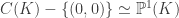$C(K) - \{ (0,0) \} \simeq \mathbb P^1(K)$ . We explain why. Define the map $phi: C(K) - \{ (0,0) \} \to \mathbb P^1(K)$ as that which sends $(x,y) \mapsto (x : y)$ . We’ll come back to this point later. Given any 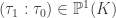$(\tau_1 : \tau_0) \in \mathbb P^1(K)$ , the intersection with the curve $C$ and the line 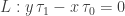$L: y \, \tau_1 - x \, \tau_0 = 0$ yields the point
$(x,y) = \left( \dfrac {\tau_1 \, (\tau_1^2 - \tau_0^2)}{(\tau_1 - 2 \, \tau_0) \, (\tau_1^2 + \tau_0^2)}, \ \dfrac {\tau_0 \, (\tau_1^2 - \tau_0^2)}{(\tau_1 -2 \, \tau_0) \, (\tau_1^2 + \tau_0^2)} \right).$
(Actually, $(x,y) = (0,0)$ corresponds to $(\tau_1 : \tau_0) = (\pm 1 : 1)$ so we get all of the points on $C$ , but the map fails to be one-to-one at this point.) In particular, the nonsingular points $C(K) - \{ (0,0) \} \simeq \mathbb P^1(K)$ form a curve of genus $g(\mathbb P^1) = 0$ — even though $C$ is a curve of degree $d = 3$ . This means the genus formula we introduced before does not work when the projective curve is singular.

We will discuss more examples in the next lecture.

S	M	T	W	T	F	S
				1	2	3
4	5	6	7	8	9	10
11	12	13	14	15	16	17
18	19	20	21	22	23	24
25	26	27	28	29	30	31